It’s a common scenario: a business wants to run complex queries on its production database to harness fresh, operational data.
This makes sense, since some of the most vital data is held on these databases, including transactions, payments, and inventory. The data is also fresh, allowing you to power operational use cases.
However, most of this data is held in databases that are not designed to process this complex query load. As a result, the database strains and becomes unstable. Results take longer to generate, and they become out-of-date.
This is where an operational data store (ODS) comes in. An operational data store allows you to perform complex queries on fresh data, without performance or stability issues. Teams can power their operational use cases, instead of using traditional databases that can’t handle the query load.
To showcase the power of an ODS, we’ve developed a demo for an e-commerce company, based on a dynamic pricing use case. Read on for a step-by-step walkthrough.
What is an ODS?
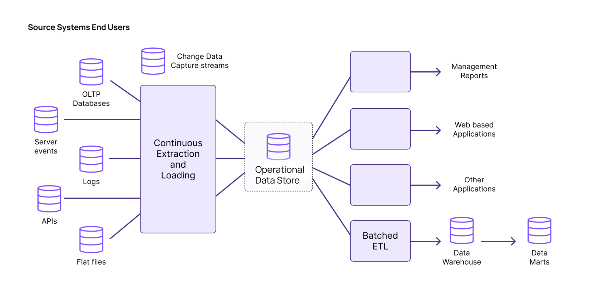
An operational data store (ODS) offers the best of both worlds: the ability to process data intensive queries like a data warehouse, but with fresh results, like OLTP. Teams can model everything in SQL, and easily manipulate streams of data.
While OLTP is built for fresh results, and OLAP is designed for data intensiveness, ODS does both at the same time. When query loads become too heavy for OLTP, ODS allows teams to perform complex queries on fresh data to power operational use cases, such as fraud detection and personalization.
An ODS works natively on Change Data Capture (CDC) streams from the transactional database. Data from OLTP databases is incorporated within milliseconds, so that the results from the ODS are always fresh.

An ODS can easily handle data intensive workloads, such as joins from normalized tables upstream. ODS also incrementally updates your views as data comes in, ensuring that you don’t use excessive compute.
Demo Use Case: Operational Data Store
We recently developed a demo to showcase Materialize’s ODS in action. In the demo, the e-commerce company Freshmart is trying to incorporate dynamic pricing into its website.
Dynamic pricing allows prices to vary based on a number of factors, including stock levels, trends, and other indicators. The dynamic pricing logic is represented by a single, complex SQL query.
Freshmart has created foreign key constraints and indices to speed up queries as much as possible, but these methods still aren’t enough.
ODS Demo: Step-by-Step Walkthrough
First, let’s take a look at the query for the dynamic pricing model. You can find the SQL code below.
CREATE VIEW dynamic_pricing AS
WITH
    recent_prices AS (
        SELECT
            grp.product_id,
            avg(sub.price) AS avg_price
        FROM (SELECT DISTINCT product_id FROM public.sales) AS grp,
            LATERAL (
                SELECT
                    sales.product_id,
                    sales.price
                FROM public.sales
                WHERE sales.product_id = grp.product_id
                ORDER BY sales.sale_date DESC LIMIT 10
            ) AS sub
        GROUP BY grp.product_id
    ),

    promotion_effect AS (
        SELECT
            p.product_id,
            min(pr.promotion_discount) AS promotion_discount
        FROM public.promotions AS pr
        INNER JOIN public.products AS p ON pr.product_id = p.product_id
        WHERE pr.active = TRUE
        GROUP BY p.product_id
    ),

    popularity_score AS (
        SELECT
            s.product_id,
            rank() OVER (PARTITION BY p.category_id ORDER BY count(s.sale_id) DESC) AS popularity_rank,
            count(s.sale_id) AS sale_count
        FROM public.sales AS s
        INNER JOIN public.products AS p ON s.product_id = p.product_id
        GROUP BY s.product_id, p.category_id
    ),

    inventory_status AS (
        SELECT
            i.product_id,
            sum(i.stock) AS total_stock,
            rank() OVER (ORDER BY sum(i.stock) DESC) AS stock_rank
        FROM public.inventory AS i
        GROUP BY i.product_id
    ),

    high_demand_products AS (
        SELECT
            p.product_id,
            avg(s.sale_price) AS avg_sale_price,
            count(s.sale_id) AS total_sales
        FROM public.products AS p
        INNER JOIN public.sales AS s ON p.product_id = s.product_id
        GROUP BY p.product_id
        HAVING count(s.sale_id) > (SELECT avg(total_sales) FROM (SELECT count(*) AS total_sales FROM public.sales GROUP BY product_id) AS subquery)
    ),

    dynamic_pricing AS (
        SELECT
            p.product_id,
            p.base_price,
            CASE
                WHEN pop.popularity_rank <= 3 THEN 1.2
                WHEN pop.popularity_rank BETWEEN 4 AND 10 THEN 1.1
                ELSE 0.9
            END AS popularity_adjustment,
            rp.avg_price,
            coalesce(1.0 - (pe.promotion_discount / 100), 1) AS promotion_discount,
            CASE
                WHEN inv.stock_rank <= 3 THEN 1.1
                WHEN inv.stock_rank BETWEEN 4 AND 10 THEN 1.05
                ELSE 1
            END AS stock_adjustment,
            CASE
                WHEN p.base_price > rp.avg_price THEN 1 + (p.base_price - rp.avg_price) / rp.avg_price
                ELSE 1 - (rp.avg_price - p.base_price) / rp.avg_price
            END AS demand_multiplier,
            hd.avg_sale_price,
            CASE
                WHEN p.product_name ILIKE '%cheap%' THEN 0.8
                ELSE 1.0
            END AS additional_discount
        FROM public.products AS p
        LEFT JOIN recent_prices AS rp ON p.product_id = rp.product_id
        LEFT JOIN promotion_effect AS pe ON p.product_id = pe.product_id
        INNER JOIN popularity_score AS pop ON p.product_id = pop.product_id
        LEFT JOIN inventory_status AS inv ON p.product_id = inv.product_id
        LEFT JOIN high_demand_products AS hd ON p.product_id = hd.product_id
    )

SELECT
    dp.product_id,
    round(dp.base_price * dp.popularity_adjustment * dp.stock_adjustment * dp.demand_multiplier, 2) AS adjusted_price,
    round(dp.base_price * dp.popularity_adjustment * dp.stock_adjustment * dp.demand_multiplier * dp.promotion_discount * dp.additional_discount, 2) AS discounted_price
FROM dynamic_pricing AS dp;


ALTER TABLE public.inventory ADD CONSTRAINT inventory_product_id_fkey FOREIGN KEY (product_id) REFERENCES public.products (product_id);
ALTER TABLE public.promotions ADD CONSTRAINT promotions_product_id_fkey FOREIGN KEY (product_id) REFERENCES public.products (product_id);
ALTER TABLE public.sales ADD CONSTRAINT sales_product_id_fkey FOREIGN KEY (product_id) REFERENCES public.products (product_id);

CREATE INDEX idx_products_product_name ON products (product_name);
CREATE INDEX idx_sales_product_id ON sales (product_id);
CREATE INDEX idx_sales_sale_date ON sales (sale_date);
CREATE INDEX idx_sales_product_id_sale_date ON sales (product_id, sale_date);
CREATE INDEX idx_promotions_product_id ON promotions (product_id);
CREATE INDEX idx_promotions_active ON promotions (active);
CREATE INDEX idx_promotions_product_id_active ON promotions (product_id, active);
CREATE INDEX idx_inventory_product_id ON inventory (product_id);
As you can see, the query is relatively complicated, containing complex lateral joins, group bys, aggregations, and left joins. The indexes are added to make the query run efficiently in Postgres.
Postgres will give us access to real-time data about purchases, inventory, and other vital business metrics. But Postgres will have difficulty with the complexity of the query. The query is too compute-intensive, and the OLTP architecture of Postgres will strain.
To show this in action, we’ll connect to a Postgres instance. Let’s perform the dynamic pricing query.

The output is as follows:

In our testing, performing a single query took ten seconds. However, performing ten queries concurrently took 30 seconds. Concurrent computations are likely to occur on the e-commerce website, since more than one user will shop at a time.
However, pricing that takes 30 seconds to generate is not necessarily accurate. By then, data on the site has changed, and the price may not reflect the latest information.
So if we want to perform this dynamic pricing query at an acceptable speed, we’ll have to take it off Postgres.
What other solutions could you use? A read replica allows you to unload queries off of your primary, but they’re designed for transactional queries, not analytical queries.
You could ETL the data into a data warehouse, but then the data would be stale. You could try a cache, but that pulls you away from SQL.
This is where an operational data store (ODS) comes in.
An operational data store allows you to perform this complex query over fresh business data, such as inventory levels.
For this demo, we’ll use Materialize as a cloud operational data store (ODS). Materialize allows you to use SQL to transform, deliver, and act on fast-changing data. By performing incremental and consistent data transformations, Materialize enables you to serve always-fresh query results to power real-time use cases.
To get started with Materialize, sign up for a free trial now. Then log in to the Materialize Console.
There are several ways you can bring business data into Materialize. You can read data off of Kafka, post off a Webhook, and ingest data from databases by consuming CDC data from a replication log. Learn how to import data sources into PostgreSQL by reading our documentation.
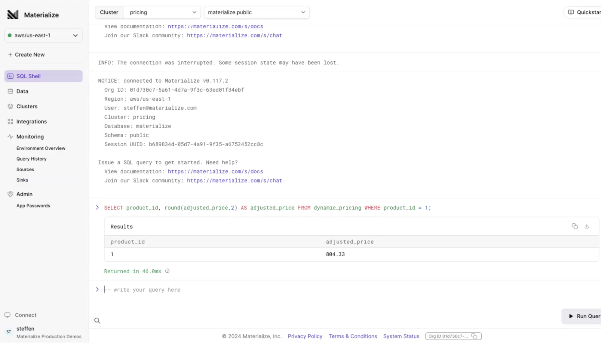
Let’s perform the same dynamic pricing query from our first example in Materialize.

In our test, Materialize provides the same answer as Postgres, but it is generated in 46 milliseconds instead of 10 seconds. This is much quicker, and takes place fast enough to serve as accurate pricing on the website.
Freshmart Demo: See Why ODS Works Best
It makes sense that many teams end up performing complex queries on databases such as Postgres. The transactional data is fresh and vital for business operations, such as purchases and account balances. But OLTP databases are ill-equipped to handle these compute-intensive queries.
That’s where the operational data store is relevant. Operational data stores such as Materialize allow you to perform complex queries on fresh data, enabling you to power operational use cases.
Sign up for a free trial of Materialize now, so you can power your real-time business use cases with a cloud ODS.


